Why we’re taking column-level lineage to the next level


Here’s a confession you might not expect from a data guy like me: I find SQL code scary.
And I’m sure I’m not the only one. Today’s modern data platforms have become so powerful that joining data across ten or fifteen tables in a single SQL query is a piece of cake. Just write the SQL, and it gets executed in seconds.
But a feature like this can be a double-edged sword.
While convenient and extremely powerful from a computation perspective, it comes with a heavy toll. Maintaining this kind of SQL code is complex. Data often flows through layers of transformations (either expressed as CTEs or nested queries), case statements, and dozens of branches joining and splitting values that are finally pulled out as a table.
WITH
active_users AS (
    SELECT
        user_id,
        first_name,
        last_name,
        email
    FROM users
    WHERE account_status = 'Active'
),
recent_purchases AS (
    SELECT
        user_id,
        order_id,
        purchase_date,
        total_amount
    FROM orders
    WHERE purchase_date >= DATEADD(month, -1, GETDATE())
),
user_spend AS (
    SELECT
        user_id,
        SUM(total_amount) AS total_spent
    FROM orders
    WHERE purchase_date >= DATEADD(month, -6, GETDATE())
    GROUP BY user_id
),
first_time_buyers AS (
    SELECT
        user_id,
        MIN(purchase_date) AS first_purchase_date
    FROM orders
    GROUP BY user_id
    HAVING MIN(purchase_date) >= DATEADD(month, -1, GETDATE())
),
repeat_customers AS (
    SELECT
        user_id,
        COUNT(*) AS orders_count
    FROM orders
    GROUP BY user_id
    HAVING COUNT(*) > 1
),
average_order_value AS (
    SELECT
        AVG(total_amount) AS avg_order_value
    FROM orders
    WHERE purchase_date >= DATEADD(month, -1, GETDATE())
),
top_selling_products AS (
    SELECT
        TOP 10 product_id,
        COUNT(order_id) AS units_sold
    FROM order_details
    GROUP BY product_id
    ORDER BY units_sold DESC
),
qualified_logins AS (
    SELECT
        user_id,
        login_date,
        DATEDIFF(minute, session_start, session_end) AS session_duration
    FROM logins
    WHERE login_date BETWEEN DATEADD(month, -1, GETDATE()) AND GETDATE()
),
active_sessions AS (
    SELECT
        user_id
    FROM qualified_logins
    WHERE session_duration > 5 -- Assuming an active session is one lasting more than 5 minutes
    GROUP BY user_id
    HAVING COUNT(*) > 1 -- User must have logged in more than once to be considered active
),
monthly_active_users AS (
    SELECT
        COUNT(DISTINCT user_id) AS MAU
    FROM active_sessions
),
customer_lifetime_value AS (
    SELECT
        u.user_id,
        u.first_name,
        u.last_name,
        ISNULL(SUM(o.total_amount), 0) AS lifetime_value
    FROM users u
    LEFT JOIN orders o ON u.user_id = o.user_id
    GROUP BY u.user_id, u.first_name, u.last_name
),
kpis AS (
    SELECT
        (SELECT COUNT(*) FROM active_users) AS active_user_count,
        (SELECT COUNT(*) FROM first_time_buyers) AS first_time_buyer_count,
        (SELECT COUNT(*) FROM repeat_customers) AS repeat_customer_count,
        (SELECT AVG(total_spent) FROM user_spend) AS avg_user_spend_last_6_months,
        (SELECT avg_order_value FROM average_order_value) AS avg_order_value_last_month,
        (SELECT MAU FROM monthly_active_users) AS monthly_active_users_count
)
SELECT * FROM kpis;
Example SQL for e-commerce KPI report (generated by ChatGPT).
This is about 100 lines of code. Could you quickly check how we calculate monthly active users (monthly_active_users_count)?
What is trivial for machines powered by carefully written and tested SQL query execution engines inside modern data platforms could be very hard to comprehend for anyone who intends to maintain and evolve such complex SQL code.
And it gets worse. Everything I described so far is just one transformation. Today’s data stacks often nest dozens of layers of such transformations between data sources and final destinations, forming intricate dependencies.
Change one line of code, and something you haven’t accounted for far downstream falls apart. Even with hours of planning, this can happen to anyone.
That’s why I find SQL code a daunting prospect. Sometimes it feels like the more you know about it, the scarier it gets.
Lineage to the rescue
To help teams manage SQL complexity, the data industry developed a relatively unified solution. Lineage is the conceptual model that connects individual transformations into a directional graph that expresses table-to-table dependencies and provides mechanisms for end users to interact with. The most typical visualization approach is a direct acyclic graph (DAG), which looks like this:
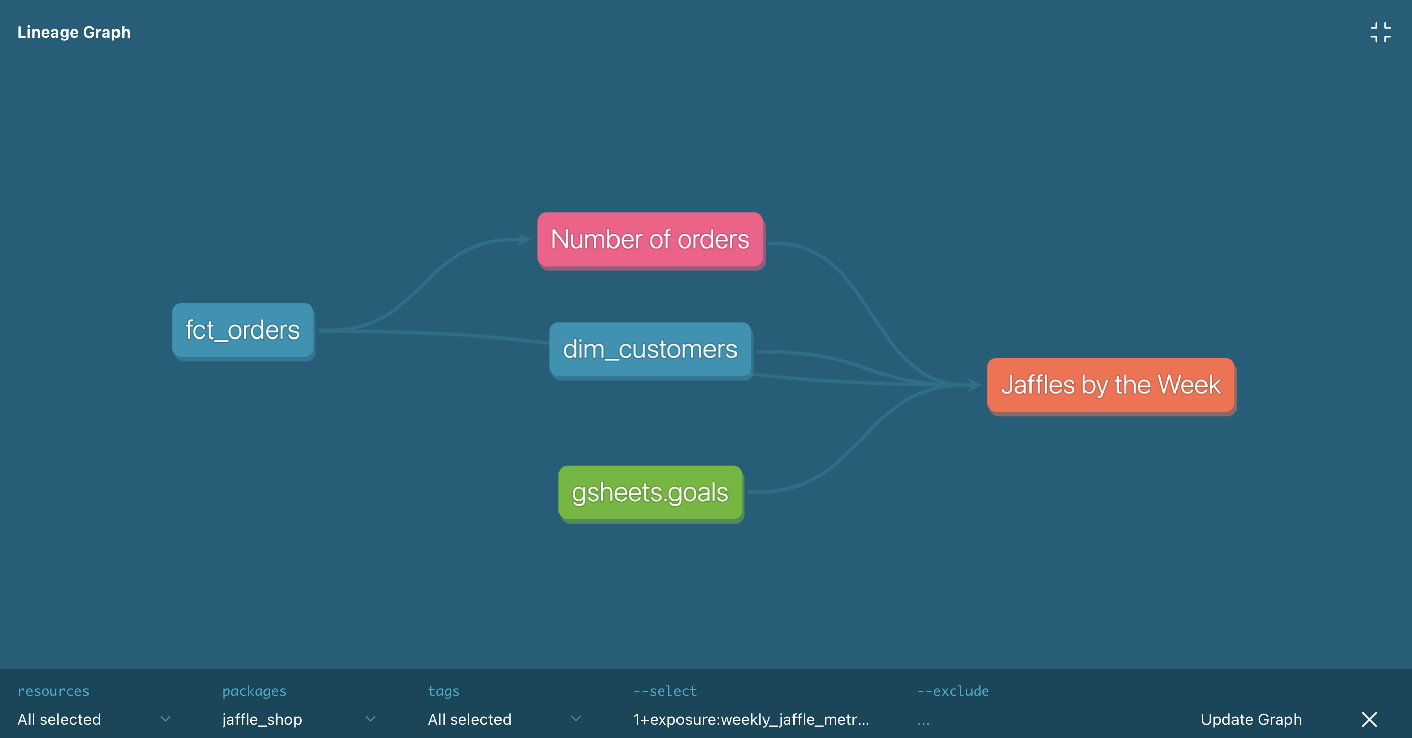
https://docs.getdbt.com/docs/build/exposures
Or if we go beyond toy examples into real-world deployments, it looks more like this:
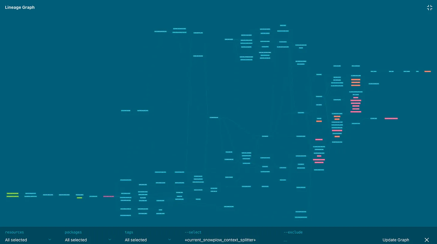
https://roundup.getdbt.com/p/complexity-the-new-analytics-frontier
However, more than a simple table-level lineage is needed despite its ability to visualize data flows through a series of models.
As data stacks grow, table-to-table lineage understanding needs to catch up.
What about the wide table with hundreds of columns in the middle of the data stack? It could easily have dozens of direct or hundreds of indirect dependencies. Do I have to review them all if I want to change one column? Manually checking every downstream model and hundreds of lines of code across them isn’t fun.
Going deeper into columns
The emergence of SQL as a de-facto standard way to query data across most modern data Platforms have opened the door for a more sophisticated solution: column-level lineage, quickly reaching many data tools, including Synq.
It requires a much more complex technology solution than table-level lineage, which can be inferred from dbt artifacts or via simple SQL code parsing.
When implementing column-level lineage at Synq, we’ve decided to go deep.
We avoided parser generators like ANTLR (more on why in the next post) and invested in handwritten lexical and syntactical analysis of SQL code. This approach opens more flexibility into the evolution of parsing logic, which can account for nuanced platform-specific SQL extensions (yes, we can understand PIVOT, too, where the entire data rotates 90 degrees and rows become columns).
We’ve invested hundreds of hours into parsing a wide range of syntax dialects and platform-specific syntax. As a result, we are excited to bring a solution to the market with broad SQL coverage across Snowflake, BigQuery, Redshift, and ClickHouse.
We’ve integrated all the above functionality into our user interface, enabling our customers to understand upstream and downstream column-level dependencies for any single column or group of columns for their tables.
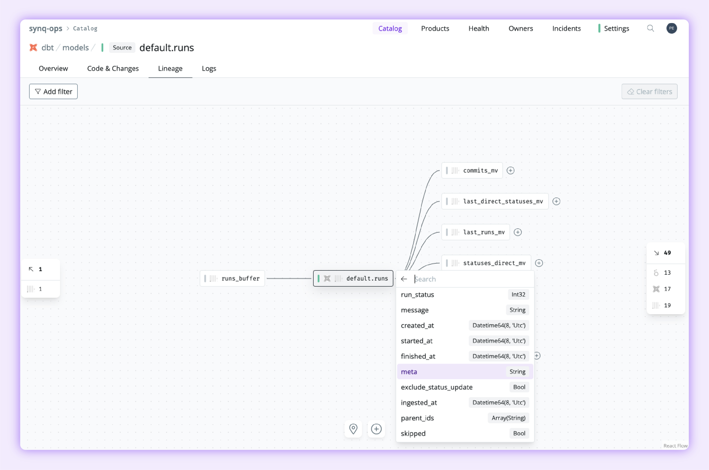
Synq column-level lineage
However, as we talked to teams, we realized that the current approach to column-level lineage still has severe limitations. While helpful in comparison to table-level lineage with its ability to provide more granular tracing of dependencies across tables, it doesn’t at all help with a critical challenge: helping teams understand SQL logic itself.
Going deeper, blending lineage and code
With column data flowing through CTEs, cases, and computation before it’s sourced from upstream tables, it still goes through non-trivial hops. So engineers are inevitably left doing a lot of scrolling up and down between relevant code snippets, often spanning hundreds of lines of code.
Inspired by tools available to software engineers, we’ve used some fundamental concepts of language parsing design to take the whole solution to the next level.
In our next post, we explain how Synq uses advanced SQL parsing to address the limitations of column-level lineage and how all of this contributes to the big picture: building integrated lineage and code interface, next-generation tooling for data practitioners.
Intrigued to see it in action? Let us know.


